CAPE crusader: advanced version

Last week I dealt with the less controversial changes to the Shiller P/E. You probably want to read that first. In this post, I derive a more advanced version: CAPE 3.0. The main finding? If you measure it differently, the last 20 years go from being an expensive aberration to a typical investment period.
Factors I adjust for:
- Average pretax earnings. I assume the future tax rate will be the same as a mixed U.S./International statutory rate +/- the difference over the previous 10 years in actual vs statutory.
- Adjust for buybacks.
- Adjust for changes in accounting standards.
- Adjust for effects during high inflation periods of overstated reported profits.
- Adjust for the cost of trading and spreads to reflect the after fee returns to shareholders
- I haven't adjusted for negative earnings. I want to see a different series that does adjust, but I don't have enough data.
- I haven't used Shiller's total return re-investment adjustment. I disagree with it.
See the effect below of this version of CAPE 3.0:
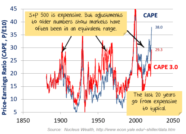
The net effect is not that much on the latest reading. But, these changes increase prior levels, in some cases substantially. Still expensive. But not outrageously so. And importantly, the last 20 years no longer look like an expensive aberration.
Relative to bonds, the excess CAPE 3.0 yield goes from slightly expensive to slightly cheap. Which probably says as much about bonds as it does equities:

The rest post is for those who care about the detail. It is probably too much information for most!
1. Tax detail
I'm going to start by admitting that I don't have 150 years of detailed company financials. There are a lot of estimates based on judgement. Hopefully, some enterprising students looking for thesis topics can fill in the gaps in the coming years.
In CAPE 2.0, I used statutory rates to adjust tax. There are so many minor tax issues that this seemed to be a less arbitrary adjustment.
In CAPE 3.0, I'm interpreting tax more realistically. First, we use the same methodology. i.e. Take an average of the last ten years of pretax profits per share then apply the current tax rate to indicate the after-tax earnings per share an investor can expect.
In this version, we use the actual tax rate paid rather than the statutory rate. This varies over time. Pre-2000s, the actual tax paid was often above the U.S. statutory rate - primarily due to the amortisation of goodwill which was not tax-deductible. Post-2000s, with no more goodwill amortisation plus the rise in international earnings and the ability of technology companies to move profits to tax havens, it is usually lower.
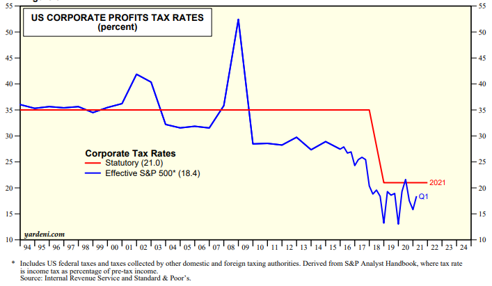
So how do investors think about it? In the 1980s, investors expected tax rates to be a little above U.S. statutory. Now they expect it below. But after the Trump tax cuts, U.S. corporate tax rates are now closer to other countries. So, the expectation should be that tax rates will not be as far below U.S. statutory as they used to be. And there needs to be some sort of transition in the numbers.
This makes for a reasonable amount of arbitrary assumptions:
- I make an estimate about the amount of tax paid internationally (very little in the mid-1900s, lots recently).
- Then make an estimate for average international tax statutory rates.
- This gives a blended statutory rate.
- I use the 10-year difference between statutory and actual tax rates as the investor's expected tax differential.
- And then I make some arbitrary changes. As you can see above, in 2008 the tax rate went to 50%+. I strip that out of investor expectations because I'm pretty sure the vast majority of investors weren't expecting that differential to return.
In most years, the net effect isn't that different from using statutory rates in CAPE 2.0. But in some individual years, it makes a difference.
2. Buyback detail
I had a few queries after my first post about the adjustment to buybacks. I want to note that this is not an adjustment for share issues. It is specific only to buybacks for the reasons below:
- When a company issues shares for an acquisition, paying down debt, or employee options, it gets something in return. i.e. work performed, an asset or a decrease in debt. The shareholder is diluted, but the intention (!) is to increase profits to compensate the shareholders. This effect is captured by earnings per share, both the numerator and denominator increase. This is an investment or operational decision.
- Buybacks are a financing decision. Whether a company chooses a buyback or a dividend does not affect the company's earnings (i.e. dollar earnings aren't affected, per share earnings might be).
- When you pay a dividend, the cash leaves the company. The shareholders get the benefit directly.
- When a buyback is performed, the cash leaves the company. Shareholders do not get cash. Shareholders get a future benefit from a reduced number of shares. This is not captured by the Shiller P/E.
A good way to think about this is to think about two different index funds which invest in the S&P500. Both funds raise $100m, invest the money in the S&P500 and issue 100m shares at $1 per share to investors in year 0:
- Dividend Fund pays out all of the dividends received to shareholders as a dividend
- Buyback Fund uses dividends received to buy back its own shares
i.e. both funds always own the same dollar amount of the underlying S&P. It is just that they both have a different number of shares in their own fund. Ideally, you want each fund to have the same valuation statistics. Using CAPE 2.0 or 3.0, they do. Using CAPE, they don't.
Say the underlying profit grows at the inflation rate. The payout ratio is 70%, and the S&P trades on 19x the prior year earnings. Then you will see the CAPE for the Buyback Fund is way higher than the other methods:
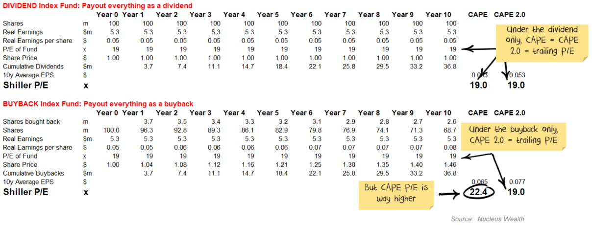
Flex the assumptions. The result is the same. Say you put in 4% real growth, under both methods CAPE 2.0 = 22.5x. The dividend only CAPE is 22.5x, but the buyback only CAPE = 26.2x.
Net Effect: because Shiller's original version does not adjust for buybacks, the CAPE will look artificially higher.
3. Asset accounting standards have changed
The main issue is this:
- In 1919 there is a pandemic, and my sales drop 50%. I write down the value of my assets by 50%. The pandemic passes, my sales bounce back, and I write the value of my assets back up.
- In 2020 there is a pandemic, and my sales drop 50%. I write down the value of my assets by 50%. The pandemic passes, my sales bounce back, and I cannot write the value of my assets back up.
Jesse Livermore does a great job of exposing these issues across a series of posts. TLDR summary: accounting standards have changed; we need to adjust earnings to reflect that.
3.1 Write-downs
Write-downs split the investment community on how to adjust. For example, a company makes $100 per year in earnings:
- It buys an asset for $50, earning $5 per year.
- Now company earnings are $105.
- Then the asset hits trouble, and the earnings fall to -$1.
- The asset gets written down to zero.
- Company earnings are $100-$1-$50 = $49 for one year and then $99 after that.
On the one hand, the $50 loss is a genuine reflection that management stuffed up. We want to see the effect, particularly if the stuff-ups are irregular but persistent. By taking a ten-year average, we get a smoothed view of the effect.
On the other hand, investors only care about the $99 and the current capital structure from a valuation perspective. That is what the company has going forward. It doesn't matter if the company paid $50 for the asset or $1 or $5,000. It was in the past. The penalty of the bad acquisition has been paid in the form of higher debt or more shares. This is the mechanism for affecting earnings per share. If we also add in the write-downs, then we are double counting. We care about how much a company that earns $99 per year is worth with today's capital structure.
3.2 Fake Write-downs
The practical problem is companies use this preference against investors. Investors want to ignore write-downs? OK, companies will try and disguise whatever they can as a write-down.
Restructuring charges pop up all the time, with companies hoping investors will ignore them. But they are not the same. Paying former employees redundancy payments is a straight-up cost, not a balance sheet adjustment. And restructuring happens all.the.freaking.time.
Companies also try other things on. Say inventory write-downs. Which sound like a real writedown. But really they simply show the company spending more on making something that it receives. Again, a straight-up loss. It isn't double counting.
3.3 No good sources of data
I've looked at company earnings data from all of the major data sources. None of them gets it right every time. Most of them make it difficult to get the actual numbers that I want. What we want to exclude are non-recurring changes in assets or liabilities. But it isn't easily available.
Mostly this is the fault of companies. They try to obfuscate. But the data collectors don't really try that hard to fix.
3.4 And in the other direction
Goodwill amortisation used to be a thing but is no more. This systematically reduced earnings before 2001, but no longer does.
That makes a difference in the opposite direction.
3.5 Pre 2000 data
I am making two assumptions that I am unsure about. One is that the write-ups will offset some (but far from all) of the write-downs. Especially as we are taking ten-year periods.
The other assumption is there were no other major accounting issues in the distant past that I should be adjusting for. I have less faith in this assumption.
3.6 Effect of changes
I have adjusted to remove 50% of the effect of write-downs from numbers post the FAS 142 accounting change.
Why only 50%? Because there were still some write-downs before 2001 (offset by write-ups). Plus goodwill amortisation. Plus, there is likely a chunk of real depreciation or amortisation that companies hide in the write-down process.
Ideally, I would prefer to see the entire time series with non-recurring changes in assets or liabilities removed. But I don't have the data.
The main effect of this is to reduce the earnings effects of the most recent crises: 2001/2002, 2008 and 2020.
4. Depreciation
Depreciation typically understates the amount of capital that a company needs to replace because of inflation. i.e. depreciation of a factory is based on the cost of building a factory, say ten years ago, rather than the cost of building the same factory today.
In particular, in times of high inflation, earnings can be considerably overstated. Jesse Livermore once again does a sterling job in his earnings mirage piece, noting:
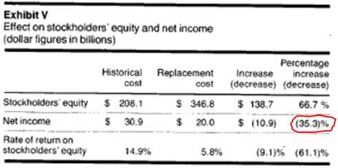
In 1977, Harvard Business Review shared the results of a review of required replacement cost disclosures of the 100 largest U.S. companies at the time. The results revealed that earnings numbers measured using a replacement cost framework were 35% lower than officially reported GAAP earnings numbers, reflecting an overstatement of 50%:
...when inflation was at its peak in the United States, [regulatory] bodies did mandate practices to correct for it. In 1976, the SEC published ASR 190, which required large companies to disclose what their financial numbers would have come out to under a replacement cost framework. FASB followed up in 1979 with the now superceded FAS 33, which required a similar disclosure.
If inflation and capital expenditure were consistent over time, then this wouldn't matter. But they aren't.
In times of high inflation (like the 1970s), earnings will be more overstated than other times. And that matches with the data - if you look at the CAPE ratio, you can clearly see high inflation periods correspond with a low apparent P/E.
This is a reflection that investors aren't stupid. They knew about these issues! In fact, the SEC issued several changes to accounting standards to require companies to disclose the difference. The S&P 500 traded on a lower P/E because investors knew the earnings were overstated.
A secondary issue is that capital expenditure has been falling as the economy changes from more manufacturing to more services. Earnings from a market that has less manufacturing and more services should be less understated.
So, I make two adjustments:
- For 10 year average inflation between 1% and 3% I make no changes. Outside that range, I use Jesse's estimates to normalise earnings back to a 2% inflation rate. Where I can (back to 1947), I calculate the inflation from capital expenditure inflation rather than consumer inflation.
- I make a small adjustment to historical earnings to reflect the rise of services and the decrease in capital expenditure.
The net effect of these changes is to increase the CAPE during periods of high inflation, in particular the 1970s.
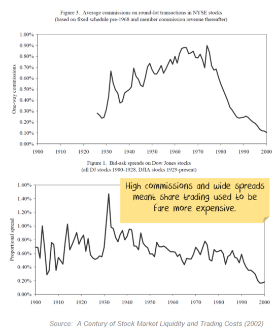
5. Cost of trading and spreads
The other major factor that changes as we look across long periods of time is the cost of investment. These days fees are sub 0.1%. Fifty years ago, investors paid significantly more, maybe 2% or more.
How does this affect valuations? Do investors price stocks based on returns before trading costs or after? I find the case more compelling that investors care about returns after trading costs.
But how much should we adjust? Sure, costs might have been 2% to buy or sell a stock, but investors traded much less. i.e. it wasn't 2% per annum. Maybe it was 2% over 2 years, or 3?
Trading volumes give some guidance, but how do we treat financial manias like the late 1920s when trading volumes rocketed?
And then you run into the issue of diversification. The only free lunch in investing. It is much cheaper and easier to get a diversified portfolio today. So it makes sense that if investors get better risk-adjusted returns, they can afford to pay more for individual stocks now than in the 1800s.
I don't know how large these adjustments should be. I have bundled them all together into a 1.25% per annum adjustment in the 1870s. I decrease this gradually to 1% in the 1970s. And then sliding roughly in line with the fall in fees to current levels. It feels about right to me, but I have no better support for these changes...
6. Negative earnings
A contentious issue.
On the one hand, share prices don't go negative. Say I have a portfolio of companies A and B making money and company C losing money:
- If A and B both make $100 and C loses $100, net earnings are $100.
- Put that on 20x earnings and my portfolio is worth $2,000
- But what happens if C goes broke? Now net earnings are $200.
- Should the value of my shares in A and B be worth more because C went broke? That doesn't make sense.
- Or is it just that my portfolio should be still worth $2,000 and it is now on 10x earnings?
At a stock level, subtracting earnings does not make sense. Maybe we should just call earnings $0 for loss-making companies?
On the other hand, there will always be some companies that lose money and others that make money. When we sum up every company in the market, we better understand the amount of money the average investor is making. i.e. someone is losing the money. When loss-making companies become a bigger part of the index, or lose more money, the index should look more expensive.
I prefer the second argument. But I do like the first as well. My preference would be to see both series. Seeing where the divergences are provides information. I have more recent data, but I don't have enough historical data to do this back in time.
7. Re-investment
There is an argument, in some circles, that if companies retain capital by paying lower dividends, future growth should be higher.
I'm not sold on this argument. If you make adjustments for lower dividends, then you also need to make adjustments for buybacks. And then, you need to make adjustments for changes in debt. And new equity issues.
My concern is that this argument conflates a financing decision with an investing decision. I believe the two are separate. For example, assume you have three companies, A, B and C. All make $100 in earnings in year 0 and want to make an investment of $75 in year 1:
- Company A pays out $25 in dividends, then retains $75 to pay for the investment
- Company B pays out $50 in dividends, buys back $50 of shares and then borrows $75 to pay for the investment
- Company C pays out $100 in dividends and then raises $75 of new shares to pay for the investment
In theory, the growth in earnings before interest and tax will be the same for all. The effect on earnings per share is different depending on interest rates, valuations and returns. But why adjust only for company A? The effect of all of the above will be captured in earnings per share.
Jesse Livermore once again did a lot of analysis to conclude that the effect was largely insignificant.
Net effect: there are different ways a company can fund growth. I don't believe dividend re-investment to be a factor worth adjusting for.
Wrap up
The messages from the CAPE 2.0 are that there are some fundamental, easily solved issues with CAPE that make it look more expensive than it is. My CAPE 3.0 changes are more arbitrary, but don't change the current levels. However, they do suggest that historical CAPE levels may have been considerably higher in some periods, considerably lower over the last 20 years.
The key message for me is that the current market is not as overvalued as the Shiller P/E makes out, and it wouldn't have to fall that far to bring it back to a more average value.
Relative to bonds, equities are a little cheap. But that probably says just as much about bonds as it does equities.
Most importantly, the last 20 years go from looking like an expensive aberration to merely being a typical investment period with some low valuations, some high.
Damien Klassen is Head of Investments at Nucleus Wealth.
Follow @DamienKlassen on Twitter or Linked In
The information on this blog contains general information and does not take into account your personal objectives, financial situation or needs. Past performance is not an indication of future performance. Damien Klassen is an authorised representative of Nucleus Wealth Management, a Corporate Authorised Representative of Nucleus Advice Pty Ltd - AFSL 515796.